
高效的 Go 二维切片分配方式及原因
/ 13 min read
Table of Contents
缘由
这篇文章来自笔者刷力扣的一点奇思妙想。以经典二维动态规划 编辑距离 为例,经常刷力扣的同学都知道,这类题目会有一个二维数组 dp,用来存储子问题的解。大部分人在写代码时,都会直接写成:
m, n := len(s1), len(s2)dp := make([][]int, m+1)for i := range dp { dp[i] = make([]int, n+1) // 在循环中每次都调用一次 `make` 来分配一个新的切片}但是,在 Effective Go 中,笔者看到一种 Go 官方推荐的做法:
If the slices might not grow or shrink, it can be more efficient to construct the object with a single allocation.
实测,这两种方式在力扣 OJ 上的运行时间差别不大,用同样的状态转移方程都可以做到 0ms 和几乎相同的内存使用。那为什么 Go 官方认为第二种方式是efficient的?
记号说明
在下文中,我们把第一种方式称为非连续布局(Separate),记作 S;第二种方式称为连续布局(Contiguous),记作 C。
直观感受
从代码上来看,
- S 布局需要调用 m+1 次 make 函数来分配内存,但每一行的切片直接指向每次 make 分配的内存块
- C 布局需要调用一次 make 函数,但需要 m+1 次切片操作来分配每一行
直觉上,make 函数的调用开销应该比切片操作大。make 函数涉及在堆上分配内存,可能有系统调用、与 GC 打交道之类的耗时指令;相比之下,Go 中的切片数据核心是指针表示,切片操作本质上是腾挪指针和修改数值,要比调用 make 函数分配内存快得多:
type slice struct { array unsafe.Pointer len int cap int}也就是说,C 布局的运行开销应该比 S 布局小。但这只是直观感受,实际情况如何呢?
Benchmark
$ go versiongo version go1.24.12 linux/amd64func allocSeparate(m, n int) [][]int { dp := make([][]int, m) for i := range dp { dp[i] = make([]int, n) } return dp}
func allocContiguous(m, n int) [][]int { dp, underlay := make([][]int, m), make([]int, m*n) for i := range dp { dp[i], underlay = underlay[:n], underlay[n:] } return dp}这两个函数是被测对象,分别对应 S 布局和 C 布局。我们用 Go 的 benchmark 工具来测试它们的性能:
func benchAlloc(b *testing.B, fn func(int, int) [][]int, m, n int) { for b.Loop() { fn(m, n) }}并设置多组方阵和非方阵测试数据,分别对应不同规模的二维切片分配。
测试数据规模
var allocCases = []benchCase{ {name: "8x8", m: 8, n: 8}, {name: "256x256", m: 256, n: 256}, {name: "1024x1024", m: 1024, n: 1024}, {name: "2048x2048", m: 2048, n: 2048}, {name: "16x4096", m: 16, n: 4096}, {name: "4096x16", m: 4096, n: 16}, {name: "128x1024", m: 128, n: 1024}, {name: "1024x128", m: 1024, n: 128},}在我的笔记本电脑上结果如下:
$ go test -bench=. -benchmem slice2d_bench_test.gogoos: linuxgoarch: amd64cpu: 13th Gen Intel(R) Core(TM) i9-13900HBenchmarkAlloc/8x8/Separate-20 3169816 364.1 ns/op 704 B/op 9 allocs/opBenchmarkAlloc/8x8/Contiguous-20 4733473 247.7 ns/op 704 B/op 2 allocs/opBenchmarkAlloc/256x256/Separate-20 7461 158784 ns/op 530818 B/op 257 allocs/opBenchmarkAlloc/256x256/Contiguous-20 10000 115274 ns/op 530820 B/op 2 allocs/opBenchmarkAlloc/1024x1024/Separate-20 445 3134147 ns/op 8415883 B/op 1025 allocs/opBenchmarkAlloc/1024x1024/Contiguous-20 1188 957516 ns/op 8415875 B/op 2 allocs/opBenchmarkAlloc/2048x2048/Separate-20 178 6883636 ns/op 33603589 B/op 2049 allocs/opBenchmarkAlloc/2048x2048/Contiguous-20 421 2802231 ns/op 33603585 B/op 2 allocs/opBenchmarkAlloc/16x4096/Separate-20 10000 110743 ns/op 524675 B/op 17 allocs/opBenchmarkAlloc/16x4096/Contiguous-20 10000 109354 ns/op 524676 B/op 2 allocs/opBenchmarkAlloc/4096x16/Separate-20 3994 257603 ns/op 622593 B/op 4097 allocs/opBenchmarkAlloc/4096x16/Contiguous-20 7003 169511 ns/op 622593 B/op 2 allocs/opBenchmarkAlloc/128x1024/Separate-20 3309 333657 ns/op 1051779 B/op 129 allocs/opBenchmarkAlloc/128x1024/Contiguous-20 3816 334851 ns/op 1051778 B/op 2 allocs/opBenchmarkAlloc/1024x128/Separate-20 5060 317356 ns/op 1075843 B/op 1025 allocs/opBenchmarkAlloc/1024x128/Contiguous-20 8068 335319 ns/op 1075842 B/op 2 allocs/op测试的结论几乎也能支持我们的直观感受:C 布局的每一轮分配总时长,几乎都比 S 布局短,在 1024x1024 方阵上二者的运行时间比甚至达到了 1: 3.3。而最终分配的内存大小相同。
有意思的现象:
-
行较少时两个布局分配速率差距不大;行越多,C 布局的优势越明显。 为了验证这个现象我又跑了另一组测试,结果如下:
行数不同,但列数相同的 Benchmark 数据
Terminal window $ go test -bench=. -benchmem slice2d_row_test.gogoos: linuxgoarch: amd64cpu: 13th Gen Intel(R) Core(TM) i9-13900HBenchmarkAlloc2/8x256/Separate-20 224769 4841 ns/op 16576 B/op 9 allocs/opBenchmarkAlloc2/8x256/Contiguous-20 320248 3751 ns/op 16576 B/op 2 allocs/opBenchmarkAlloc2/64x256/Separate-20 25479 44895 ns/op 132864 B/op 65 allocs/opBenchmarkAlloc2/64x256/Contiguous-20 43257 25004 ns/op 132864 B/op 2 allocs/opBenchmarkAlloc2/256x256/Separate-20 7269 167081 ns/op 530819 B/op 257 allocs/opBenchmarkAlloc2/256x256/Contiguous-20 10000 125339 ns/op 530819 B/op 2 allocs/opBenchmarkAlloc2/512x256/Separate-20 3498 346581 ns/op 1062147 B/op 513 allocs/opBenchmarkAlloc2/512x256/Contiguous-20 4718 360690 ns/op 1062146 B/op 2 allocs/opBenchmarkAlloc2/1024x256/Separate-20 1170 944792 ns/op 2124421 B/op 1025 allocs/opBenchmarkAlloc2/1024x256/Contiguous-20 1581 709891 ns/op 2124418 B/op 2 allocs/opBenchmarkAlloc2/2048x256/Separate-20 798 1510245 ns/op 4243460 B/op 2049 allocs/opBenchmarkAlloc2/2048x256/Contiguous-20 2485 880432 ns/op 4243460 B/op 2 allocs/opBenchmarkAlloc2/4096x256/Separate-20 380 3113531 ns/op 8486916 B/op 4097 allocs/opBenchmarkAlloc2/4096x256/Contiguous-20 1455 815917 ns/op 8486915 B/op 2 allocs/op结果从趋势上支持我们的结论。
-
1024x128的非方阵,C 布局的分配速率反而比 S 布局慢。对这个点,C 布局和 S 布局分别测试 20 次并分析,结论是:总体上这个测试点的 C 布局的运行时间更短;但 C 布局存在明显的阶段性波动。Alloc/1024x128/Separate-20 360.9µ ± 3%Alloc/1024x128/Contiguous-20 252.1µ ± 27%C 布局的波动数据
Terminal window BenchmarkAlloc/1024x128/Contiguous-20 4498 224941 ns/op 1075849 B/op 2 allocs/opBenchmarkAlloc/1024x128/Contiguous-20 4450 245386 ns/op 1075843 B/op 2 allocs/opBenchmarkAlloc/1024x128/Contiguous-20 4822 233398 ns/op 1075844 B/op 2 allocs/opBenchmarkAlloc/1024x128/Contiguous-20 7161 243204 ns/op 1075845 B/op 2 allocs/opBenchmarkAlloc/1024x128/Contiguous-20 4740 244807 ns/op 1075842 B/op 2 allocs/opBenchmarkAlloc/1024x128/Contiguous-20 4336 250888 ns/op 1075842 B/op 2 allocs/opBenchmarkAlloc/1024x128/Contiguous-20 4953 266640 ns/op 1075842 B/op 2 allocs/opBenchmarkAlloc/1024x128/Contiguous-20 3746 299419 ns/op 1075842 B/op 2 allocs/opBenchmarkAlloc/1024x128/Contiguous-20 4813 251891 ns/op 1075842 B/op 2 allocs/opBenchmarkAlloc/1024x128/Contiguous-20 5493 269371 ns/op 1075842 B/op 2 allocs/opBenchmarkAlloc/1024x128/Contiguous-20 4380 252351 ns/op 1075842 B/op 2 allocs/opBenchmarkAlloc/1024x128/Contiguous-20 4200 251041 ns/op 1075842 B/op 2 allocs/opBenchmarkAlloc/1024x128/Contiguous-20 3753 329978 ns/op 1075841 B/op 2 allocs/opBenchmarkAlloc/1024x128/Contiguous-20 4107 342029 ns/op 1075841 B/op 2 allocs/opBenchmarkAlloc/1024x128/Contiguous-20 3460 336196 ns/op 1075842 B/op 2 allocs/opBenchmarkAlloc/1024x128/Contiguous-20 3196 354317 ns/op 1075842 B/op 2 allocs/opBenchmarkAlloc/1024x128/Contiguous-20 3277 329774 ns/op 1075841 B/op 2 allocs/opBenchmarkAlloc/1024x128/Contiguous-20 3519 319312 ns/op 1075842 B/op 2 allocs/opBenchmarkAlloc/1024x128/Contiguous-20 4898 247599 ns/op 1075842 B/op 2 allocs/opBenchmarkAlloc/1024x128/Contiguous-20 4323 251800 ns/op 1075842 B/op 2 allocs/op
动态分析
采样
首先分别跑两个测试用例,2048x2048 方阵,各跑 500 轮:
$ go test -run=^$ -bench='^BenchmarkAlloc/2048x2048/Contiguous$' -benchtime=500x -count=1 -cpuprofile=cpu_c2048.out -memprofile=mem_c2048.out -o bench_c2048.test
$ go test -run=^$ -bench='^BenchmarkAlloc/2048x2048/Separate$' -benchtime=500x -count=1 -cpuprofile=cpu_s2048.out -memprofile=mem_s2048.out -o bench_s2048.test
S 布局用时 3.51s,C 布局用时 1.81s,与之前结论一致。(但这部分差别并不大,,也就是,在这个量级下每一轮的差距大约 3 毫秒。这可能也是力扣 OJ 上看不出差别的原因)
调用链分析
祭出我们的大杀器 pprof,分析调用链上最耗时的函数,使用 -flat 参数分析函数自身耗时情况:
$ go tool pprof -top -flat ./bench_s2048.test cpu_s2048.outFile: bench_s2048.test flat flat% sum% cum cum% 1.58s 32.99% 32.99% 1.58s 32.99% runtime.memclrNoHeapPointers 0.25s 5.22% 38.20% 0.25s 5.22% runtime.madvise 0.24s 5.01% 43.22% 0.24s 5.01% runtime.(*mcentral).partialSwept (inline) 0.22s 4.59% 47.81% 0.22s 4.59% runtime.procyield 0.18s 3.76% 51.57% 0.97s 20.25% runtime.(*sweepLocked).sweep 0.13s 2.71% 54.28% 0.13s 2.71% internal/runtime/atomic.(*Uint32).Add (inline) 0.13s 2.71% 56.99% 0.18s 3.76% runtime.(*spanSet).push 0.12s 2.51% 59.50% 0.12s 2.51% runtime.headTailIndex.head (inline) 0.10s 2.09% 61.59% 0.10s 2.09% runtime.(*gcBitsArena).tryAlloc (inline) 0.10s 2.09% 63.67% 0.11s 2.30% runtime.(*pallocBits).summarize 0.08s 1.67% 65.34% 0.31s 6.47% runtime.(*mheap).freeSpanLocked 0.08s 1.67% 67.01% 0.08s 1.67% runtime.(*mspan).base (inline) 0.07s 1.46% 68.48% 0.07s 1.46% runtime.futex (......)go tool pprof -top -flat ./bench_c2048.test cpu_c2048.outFile: bench_c2048.test flat flat% sum% cum cum% 1.56s 80.00% 80.00% 1.56s 80.00% runtime.memclrNoHeapPointers 0.07s 3.59% 83.59% 0.07s 3.59% runtime.madvise 0.02s 1.03% 84.62% 0.02s 1.03% runtime.(*mheap).setSpans 0.02s 1.03% 85.64% 0.02s 1.03% runtime.(*unwinder).resolveInternal 0.02s 1.03% 86.67% 0.02s 1.03% runtime.forEachPInternal 0.02s 1.03% 87.69% 0.02s 1.03% runtime.futex (......)观察到两个有意思的现象:
-
两边的耗时大头都是
runtime.memclrNoHeapPointers,这是 Go 运行时在清理内存,代表着新内存的分配。但两种布局的耗时分别为 1.56s/1.58s,差距不大。这说明,C 布局的优势并不在于初始化内存的速度。(顺带一提,这个函数在源码中是用汇编指令写就的) -
虽然
runtime.memclrNoHeapPointers在两种布局上运行时间相近,但 S 布局上其比例仅占 32.99%,C 布局上占时长比例高达 80.00%,说明另有其他耗时部分影响了 S 布局。对比上面两个 top 的结果,结合 S 布局的调用图
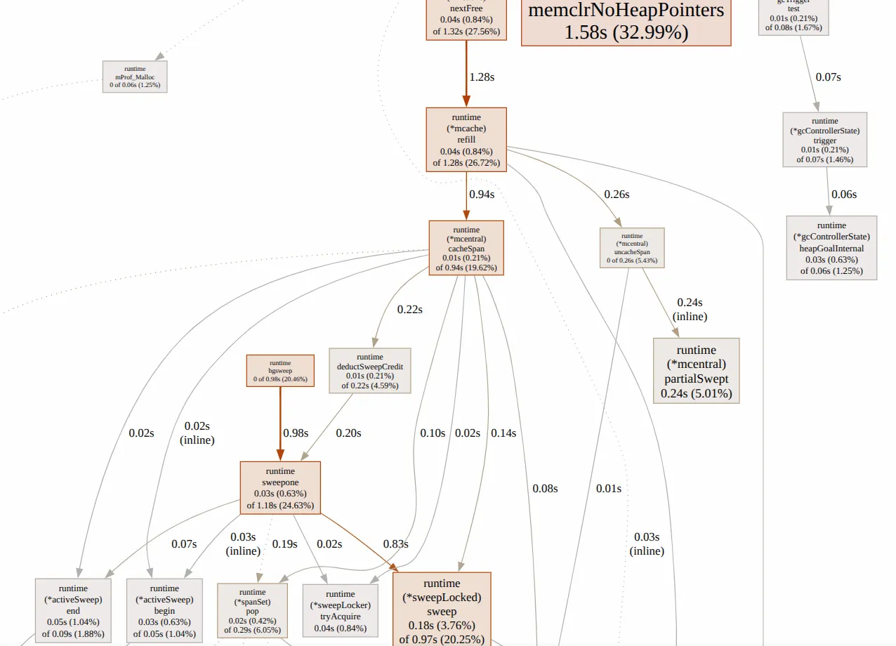 (由
(由 go tool pprof -http=:8090 ./bench_s2048.test cpu_s2048.out生成)可以看出,S 布局的
runtime.madvise(向操作系统归还内存)、runtime.(*sweepLocked).sweep(并发清扫函数,GC 的一个步骤)等函数耗时明显高于 C 布局。也就是说,S 布局的额外开销更多在于 GC、分配器 相关的函数。
结论
到这里,结论就明确了:C 布局相对于 S 布局的优势,并非初始化内存的开销——其在两种布局中相近——而在于 GC、分配器的开销更低。
Go 的 GC 和分配机制比较复杂、这些性能测试中两种函数也经常出现在同一调用链、相互影响,不能直接说 GC 和分配哪个热。但如果要再细化一些,单从耗时来看,S 布局的 GC sweep 相关函数(sweepLocked.sweep 下游调用累计 20.25%)要高于分配内存相关函数(mheap.allocSpan 下游调用累计 6.89%)。
但 C 布局也有使用限制。一个是
If the slices might not grow or shrink
这个前提条件不满足,那就不适合使用 C 布局了。所以本文 C 布局的例子就是二维 DP,数组大小是固定的;Effective Go 的例子也是一个固定大小的图片-像素处理。
另一个是官方推荐写法的小问题:
dp[i], underlay = underlay[:n], underlay[n:]得到的 dp[i] 的容量是 underlay[:n] 的容量,而不是 n;如果用
dp[i], underlay = underlay[:n:n], underlay[n:]就是 n 了。
讨论
浅显的汇编分析
之前提过「切片操作本质上是腾挪指针」,并没有在上述测试中体现出来。
使用 $ go tool objdump -s "allocContiguous" bench_c2048.test 来查看汇编指令,在 dp[i], underlay = underlay[:n], underlay[n:] 这一行,让 AI 大人帮笔者查阅(因为对汇编知之甚少),确实是在做我们的切分操作,包括计算指针地址、修改切片的 len 和 cap 等等。
命名严谨吗?
虽然看上去,S 布局是分配随机内存、「非连续」的,但笔者做过实测,打印每一行的地址,其依然可能连续。256、1024 大小的切片,分配的内存地址是连续的;而 1433 这样大小的切片,分配的内存地址就不连续了。这是否是语言层面的保证,还是本机特性,值得一篇新的博客挖坑。总之,S 布局不一定是非连续的,但 C 布局一定是连续的。
波动
似乎有一些矩阵规格存在阶段性波动,比如先前所述 1024x128,原因未知。挖坑